The big O notation (also asymptotic notation) helps determine how a function may decline or scale with a larger set of inputs (n). According to Wikipedia,
It is a mathematical notation that describes the limiting behavior of a function when the argument tends towards a particular value or infinity Wikipedia
Its role in helping decide how a program/function can scale is why it’s important for software writers to have a proper understanding of it. Unfortunately, people ignore the basics of computer science as soon as they understand the syntax of a language they program in. Even worse, developers do not think of future failure possibilities of code they’ve written as long as it works in the moment they need it. Most people have abused the term MVP (Minimum Viable Product) to describe the big ball of mud they write.
The big O is derived from the word “Order” which is the rate of growth of a function in computer science and there’s also a little o (another landau’s symbol) which has its applications in math.
Here’s a list of common function orders starting with slow growing functions:
| Notation | Name |
|---|---|
| 0(1) | Constant |
| 0(log(n)) | Logarithmic |
| 0((log(n))c) | Polylogarithmic |
| 0(n) | Linear |
| 0(n2) | Quadratic |
| 0(nc) | Polynomial |
| 0(cn) | Exponential |
| 0(n!) | Factorial |
An important part to note here is a O(log(nc)) is the same as O(log(n)). The big O will ignore the fact that the value being passed to a logarithmic function is changed. That can be clearly seen from here:
f(x) = log(x^2)
The input is evaluated at the logartihmic level before being evaluated by the main function order so
f(3) = log(3)
would have the same functional complexity as
f(3) = log(3^3)
f(3) = log(21)
Also worth considering is that while O(cn) may look a lot like O(nc), it grows a lot faster. A function that grows faster than any power of n is called a superpolynomial and one that grows slower than an exponential function (nc) is called subexponential.
Consider the JavaScript function here:
const getCube = (n) => n ** 3No matter what input (n) is passed to the getCube function it performs one simple function which is to find the cube root. However with a function like this:
const getPowerofThree = (n) => 3 ** nFor the first example, we will always have n * n * n but with the second it could be n * n * n * n * n ...... * n(1000th) which would consume more computational time.
Note however that the both functions getCube() and getPowerofThree() are of constant time complexity. They simply describe the operational difference of both orders O(nc) and O(cn).
We study space-time complexity of a function to understand efficiency and scalability of a piece of code. Some important resources that can be influenced by the efficiency of an algorithm are:
- CPU/Time consumption
- Memory consumption
- Energy/Power consumption
- Disk usage
- Network usage
With space (Memory consumption) and Time (CPU time to run/execute) being often the most critical. However the best algorithms really depends on what measure of efficiency is really important to the implementation.
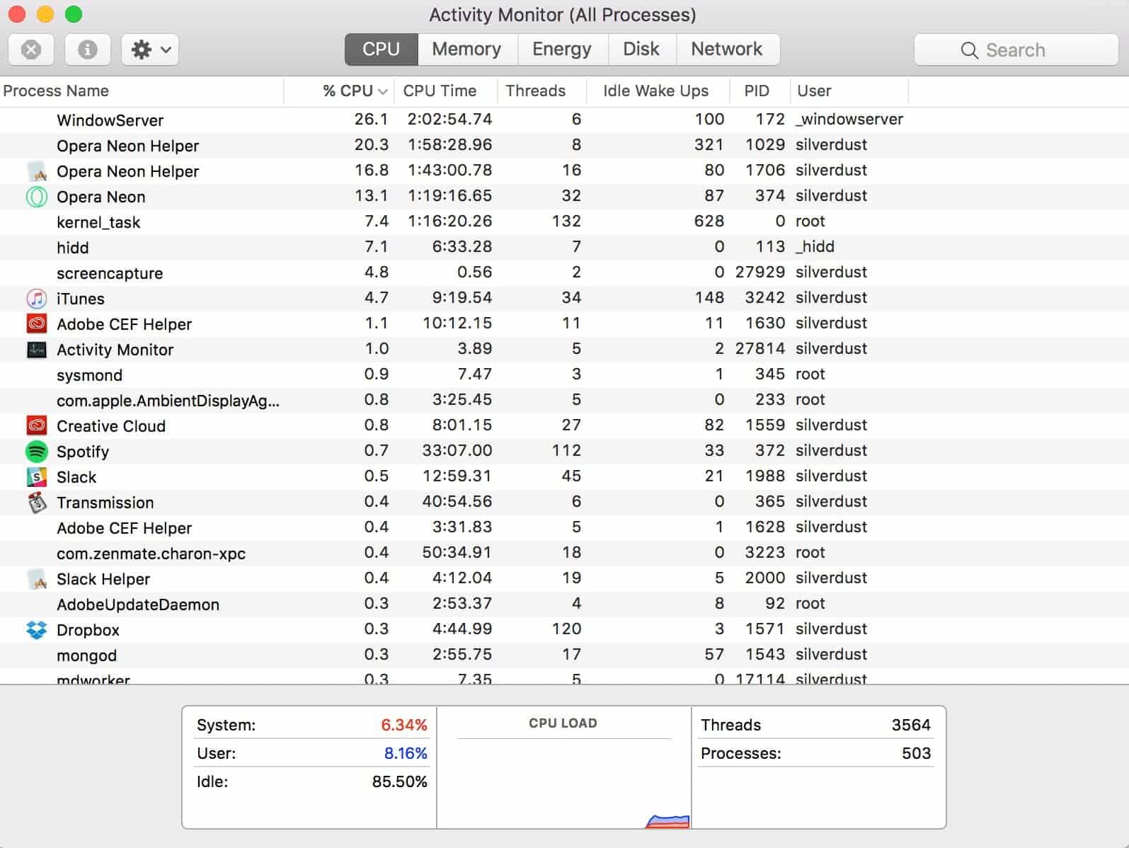
If you are on macOS you’d notice that the activity monitor basically watches for these things in programs.
Examples of the listed common notations
O(1) as the slowest growing function can be found in simple cases like checking conditions.
const input = true;
const isTrue = (bool) => bool === true;
bool(input);
Another example is the use of a dictionary/Hashmap to return a value based on its key as input:
const getHex = (color) => {
  colorDictionary = {blue: '#00f', red: '#f00', green: '#0f0'}
  return colorDictionary[color];
};
I could rewrite the getHex() function in an uglier code structure using massive ifs.
const getHex = (color) => {
  let hex;
  if(color == 'blue'){
    hex = '#00f';
  }else if(color == 'red'){
    hex = '#f00';
  }else{
    hex = '#0f0';
  }
};
but note here that the operation remains a constant and the only difference is the brevity and neatness that comes with having it written as a Hashmap.
O(n) Simple loops are good examples of linear complexity. A loop is passed an input (n) to execute n number of times.
Looking at a simple FizzBuzz solution where n = 100:
const fizzBuzz = (n) => {
  for(let i = 0; i <= n; i++){
    let f = i % 3 == 0, b = i % 5 == 0;
    console.log(f ? b ? 'FizzBuzz' : 'Fizz' : b ? 'Buzz' : i);
  }
}
A great way to think about the complexity of function is to consider how the time required to compute a function scales with larger inputs. In a order O(n) for example, the time for computation continually scales based on the input. We had 100 as the input (n) above. To write the same function for a input f(200), the time will increase linearly with the input growth.
Sequence of statements
In a function with condition blocks of different statement complexity, the total time is found by adding the times for all statements.
function getHex(color){
  const colors = [['blue', '#00f'], ['red', '#f00'], ['green', '#0f0']];
  let hex;
  if(color == 'turquoise'){
    hex = '#00e5ee';
  }else{
    colors.forEach((val) = {
      hex = val == _.first(color) ? _.last(color) : '#000';
    });
  }
  return hex;
}
Total time = time(first statement) + time(second statement) + .... + time(nth statement)As the first block is O(1) and the second O(n) we get O(1) + O(n) which sums up as O(n). The addition of both possibilities gives the worst-case order.
O(n2) unlike the linear complexity, takes twice the time to compute with a given input (n). We see this in nested loops. For a given O(n):
const loop = (n) => {
  for(let i = 0; i < n; i++){
    console.log(i);
  }
}
when an inner loop is provided, for every loop of x there’s y number of loops.
const loop = (n) => {
  for(let x = 1; x <= n; x++){
    for(let y = 1; y <= (n - 1); y++){
      console.log(x,y);
    }
  }
}
which makes statements in the inner loop execute x * y times. The example nested loop above will execute 3 * 2 = 6 times. Hence a quadratic order O(n2).
with a deeper loop inception we get a faster growing polynomial notation O(nc).
O(log(n)) logarithmic order is not common in simple programs but an example of it is a binary search. Here’s a simple example in JavaScript
const a = [1, 2, 4, 6, 1, 100, 0, 10000, 3];

a.sort(function (a, b) {
  return a - b;
});

const binarySearch = (arr, i) => {
  const mid = Math.floor(arr.length / 2);
  console.log(arr[mid], i);

  if (arr[mid] === i) {
    console.log('match', arr[mid], i);
    return arr[mid];
  } else if (arr[mid] < i && arr.length > 1) {
    console.log('mid lower', arr[mid], i);
    return binarySearch(arr.splice(mid, Number.MAX_VALUE), i);
  } else if (arr[mid] > i && arr.length > 1) {
    console.log('mid higher', arr[mid], i);
    return binarySearch(arr.splice(0, mid), i);
  } else {
    console.log('not here', i);
    return -1;
  }

}
binarySearch(a, 100);
Binary Search Example Source Visual binary search operation
We may begin to write more efficient software with slower growing functions but this wouldn’t always cover every part of performance of a software. For a complete performance check, you also need to consider the hardware resources the program is being run against e.g processing capability, also compiler/interpreter speed. With more performance needs, multithreading becomes significantly needed and that’s where languages with immutable data and static types shine.
Here are some useful resources to learn more on algorithms and complexity theory: